A Semantic Layer That Reads as SQL

Why a cube definition should be an executable query — not a YAML description of one. And what AI has to do with it.

Ten versions of the truth

Every sufficiently large company has lived through the same conversation. The CFO asks, "What was our revenue this quarter?" — and gets three different answers from three different analysts. Not because anyone made a mistake. One counted revenue with VAT, another without, a third excluded returns but included intercompany sales.

The data, meanwhile, sits in one place — ClickHouse, BigQuery, Snowflake, or another analytical warehouse. The problem isn't the data. The problem is that the definition of a metric — what "revenue" means, how sales relate to stores, who is allowed to see which regions — doesn't live in one place. It lives in analysts' heads and in hundreds of scattered SQL queries.

And business users end up in Excel anyway. You rolled out dashboards, bought licenses, ran trainings, built self-service portals — and still, every report ends its life as an Excel export on someone's desktop. That's not a failure of your team; it's how people actually work. Meanwhile, between Excel and the warehouse grows a pipeline of CSV exports and "intermediate" files, each one another opportunity for the numbers to drift apart.

This is exactly the problem a semantic layer solves: define your metrics once, under IT control with fine-grained access — then let thousands of users explore them and get the same numbers. Excel becomes the front end. Your warehouse stays the single source of truth.

A beautiful idea. So why do so many semantic layer projects stall at the pilot stage?

Why data teams struggle with semantic layers

Ask a data engineer what a semantic layer is, and the answer will depend on whose documentation they read last. The term is overloaded: metrics layer, headless BI, semantic layer, universal semantic layer — every vendor defines it differently and draws its own architecture diagram. A team reads three articles and comes away with three different pictures of the world.

Then it turns out that a semantic layer is, as a rule, a separate system with its own lifecycle. Its own modeling language to learn. Its own compiler to run. Its own deployment process, its own versions, its own breaking changes. The "warehouse + orchestrator + BI" stack gains yet another moving part that has to be studied, upgraded, and fixed.

The cost of entry before the first result turns out to be high. Before the business sees a single number, someone has to design the model, absorb a new vocabulary — semantic models, entities, measures, metrics, with metrics further split into types: simple, ratio, derived, cumulative — wire up integrations, and explain to everyone why any of this was necessary. That's weeks of work before the first "wow," and an organization's budget of patience is not unlimited.

Finally, the layer often has no obvious owner. Analysts consider it infrastructure ("that's for the engineers"), engineers consider it analytics ("that's about business metrics"). The layer hangs between teams, and once the enthusiasm of the first sprint wears off, nobody is left to maintain it.

None of this says the idea of a semantic layer is bad. All of it says one thing: the cost of adoption of a typical implementation is too high. Let's see where that cost comes from.

How it's done today: YAML on top of SQL

The dominant approach in modern semantic layers is declarative metadata. The model is described in YAML files: here are the entities, here are the dimensions, here are the measures, here are the metrics built on top of the measures. A dedicated engine reads these files and generates SQL at query time.

It looks roughly like this. Suppose we need one single metric — the number of units sold:

semantic_models:
  - name: sales
    description: One row per sale
    model: ref('fct_sales')
    defaults:
      agg_time_dimension: sale_date
    entities:
      - name: sale
        type: primary
        expr: sale_id
      - name: store
        type: foreign
        expr: store_id
    dimensions:
      - name: sale_date
        type: time
        type_params:
          time_granularity: day
    measures:
      - name: qty
        agg: sum

metrics:
  - name: sales_quantity
    label: Sales Quantity
    type: simple
    type_params:
      measure: qty

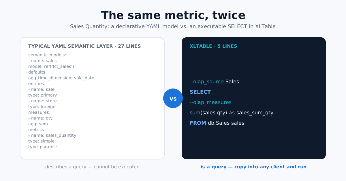
Almost thirty lines, two sections, four levels of nesting — and notice: the measure qty is not yet a metric by itself. For the user to see a number, a metric of type simple must be declared on top of the measure — one that "simply uses the measure as is."

This approach has real strengths, and they deserve an honest mention. YAML is machine-readable — convenient for building APIs and code generation on top of. A declarative model isn't tied to any particular SQL dialect. The files live happily in git. All true.

But there is a price, and here it is.

YAML cannot be executed. It is a description of a query, not a query. The debugging loop looks like this: edit the YAML → run the compiler → the engine generates SQL → execute it → get an error in the generated SQL → mentally translate it back to lines of YAML that don't exist in that SQL. Every iteration passes through a layer of indirection. The engineer debugs something other than what they wrote.

The SQL never went away — it just moved into string literals. As soon as an expression gets any more complex than a sum over a column, an expr field appears in the YAML with a chunk of SQL inside: expr: case when status = 'closed' then amount end. You get the worst of both worlds: expressions are still written in SQL, but now they live inside YAML strings — no syntax highlighting, no validation, with escaping rules and multi-line blocks via |. Some systems add a templating engine on top — and now you have Jinja inside YAML inside SQL.

Every tool is a new system of concepts. Entities with types primary/foreign/unique/natural, dimensions with type_params, metrics of four kinds — each vendor has its own ontology, and none of it transfers between tools. Unlike SQL, which every person on a data team already knows.

Join semantics are declared abstractly. You write type: foreign — but which JOIN the engine will actually build, and which path it will take through the model graph, only becomes visible after compilation. When the engine picks an unexpected join path, debugging turns into a study of the generator's internals.

A definition can only be validated through the toolchain. Validating a model means running the vendor's compiler with its own error messages. Without the tool installed and configured, a YAML file is just text.

Add it all up and you get exactly that high cost of adoption from the previous section. It isn't accidental — it's built into the architecture of the approach: between the engineer and their data stands a layer of abstraction that must be learned before it starts to help.

Before building XLTable, we spent years implementing and operating Microsoft Analysis Services in large retail companies — watching the business live in PivotTables while IT lived in cube definitions. XLTable grew out of that experience, not out of a desire to invent a new format. And so we took a different path.

The XLTable principle: the executable SELECT

XLTable is an XMLA-compatible OLAP semantic layer for ClickHouse, Snowflake, BigQuery, Databricks, StarRocks, Trino, Greenplum, and DuckDB. Excel sees it as a familiar OLAP cube: MDX queries, PivotTables, hierarchies — everything works just as it does with Microsoft Analysis Services (for which XLTable is a drop-in replacement). What reaches the database is already optimized SQL. No SQL for end users, no data copies. The semantic layer here is the cube definition: measures, dimensions, hierarchies, relationships, and permissions.

And that cube is defined not in YAML and not in a graphical designer, but in SQL. Here is the equivalent of those thirty lines of YAML from the previous section:

--olap_source Sales
SELECT
--olap_measures
    sum(sales.qty) as sales_sum_qty --translation=`Sales Quantity` --format=`#,##0`
FROM db.Sales sales

Five lines. But the key property isn't brevity — it's this: this is a working query. Mentally strip the comments and you're left with an ordinary SELECT that can be copied into any database client, executed, and it returns real rows. The tags in the comments (--olap_source, --olap_measures, --translation) merely tell XLTable how to assemble such queries into a cube.

We call this the executable SELECT principle, and it is not a syntactic quirk — it is the foundation of the whole system. Several things follow from it:

Debugging is execution. "Does the model compile?" is not a question that exists. The question is "does the query run" — and the database itself answers it, with an ordinary SQL error, in the dialect you write every day.

The barrier to entry is knowing SELECT. There is no ontology of entities and metric types to absorb. If an engineer can write SELECT ... FROM ... LEFT JOIN, they can define cubes. A first cube is realistically an evening's work, and the full path from installing the server to the first PivotTable in Excel takes about an hour.

Reviews work like regular code reviews. The diff of a definition reads at a glance; the reviewer sees actual SQL, not a description of SQL.

No hidden magic. The queries XLTable sends to the database are exactly the ones written in the definition, plus aggregation over the fields the user selected. Turn on logging — and you see every generated query.

A fair objection at this point: aren't the comment tags themselves a DSL? They are — any convention is. The difference is where that DSL lives. Strip every tag from an XLTable definition and the host language still executes: what remains is a valid SELECT. The surface area is a dozen tags, not an ontology of entities and four kinds of metrics. And validation doesn't depend on a proprietary compiler — the database checks the query, and XLTable checks the tags.

Anatomy of a cube

Let's walk through what a definition consists of — with examples, each of which, remember, can be executed as is.

Measures are the numbers the business wants to count. A measure is an aggregate function, an alias, and optional display tags:

--olap_source Sales
SELECT
--olap_measures
 sum(sales.qty) as sales_sum_qty --translation=`Sales Quantity` --format=`#,##0;-#,##0`
,sum(sales.sum) as sales_sum_sum --translation=`Sales Amount`   --format=`#,##0.00;-#,##0.00`
FROM db.Sales sales
LEFT JOIN db.Stores stores ON sales.store_id = stores.id

The translation tag sets the name the user sees in the Excel field list; format sets the numeric format in the PivotTable. Everything sits on the same line as the measure itself — the definition and its metadata never drift apart into separate files.

Dimensions are the context of analysis: stores, regions, products, time. Syntactically they mirror measure groups:

--olap_source Stores
SELECT
--olap_dimensions
 stores.id as stores_id
,stores.store_name as stores_name --translation=`Store`
FROM db.Stores stores

Hierarchies are parent-child relationships between attributes, so a user can drill from year to day in one click. Four tags — and the hierarchy is done:

 times.year    as times_year    --hierarchy=`Dates`
,times.quarter as times_quarter --hierarchy=`Dates`
,times.month   as times_month   --hierarchy=`Dates`
,times.day     as times_day     --hierarchy=`Dates`

Relationships between measures and dimensions are not described with abstract types — they are written as ordinary, explicit LEFT JOINs. A dimension links to a measure group through a shared table alias: if the measure group contains LEFT JOIN db.Stores stores and the dimension's source is FROM db.Stores stores, XLTable connects them on that alias. The JOIN is visible to the naked eye — what is written is what runs.

Special cases get clarifying tags. The most popular one in the ClickHouse world is one-table, for denormalized tables where measures and dimensions live in one wide table and no real JOIN is needed. There is many-to-many for classic many-to-many relationships (several managers assigned to one store) and part-source for helper lookup tables that are needed inside a single source but should not become part of the cube.

Calculated fields are virtual measures built on top of other measures — including measures from different measure groups:

--olap_cube
--olap_calculated_fields Calculated fields
(sales_sum_qty / nullIf(stock_avg_qty, 0)) as turnover --translation=`Turnover`

Here inventory turnover is computed from sales and average stock — two different fact tables. XLTable merges the per-group results with a FULL JOIN on its own; all the expression has to do is guard against division by zero.

Security — in the same file, in the same syntax

In a typical architecture, access rights live apart from the data model — in an admin panel, in separate configs, in the BI tool. In XLTable, a role is just another block of the same definition:

--olap_user_role
--olap_user_groups
finance_users
--olap_measures_visible
sales_sum_sum
--olap_dimensions_visible
Stores, Regions
--olap_access_filters
region in (`EU`, `NA`)

A role defines which measures and dimensions a user group can see, and olap_access_filters sets row-level security: the finance users in this example physically receive only rows for the EU and NA regions — the filter is baked into every SQL query the server generates for them. Groups come from Active Directory, so access is granted to directory roles rather than individuals — as it should be in the enterprise.

Crucially, all of this is part of the same text definition. Permissions go through the same code review and live in the same git history as the model itself.

When static isn't enough: Jinja

Honesty requires an admission: we have templating too. Cube definitions support Jinja — for the cases where SQL has to change dynamically: relative dates ("last 30 days" from the current moment), conditional logic, swapping a table for a pre-computed aggregate for performance.

The difference from the YAML approaches lies in the role the templating engine plays. There, the declarative layer is mandatory for every metric; here, Jinja is an optional add-on for the five percent of cases where plain SQL falls short. Our own documentation puts the recommendation plainly: use Jinja for small SQL adjustments and avoid complex logic. The core of the cube remains an executable SELECT.

What the business gets

The user-facing side of the story fits in one sentence: business users stay in Excel, and there is nothing to retrain them on. No add-ins, no plugins, no "new, more convenient interface." A native PivotTable connects to XLTable the same way it has connected to Analysis Services for twenty years — while the data lives in ClickHouse, billions of rows deep.

Two details users appreciate most.

Drillthrough. Double-click any cell in the PivotTable — and Excel shows the underlying rows that produced that number: the individual receipts, dates, stores. All of the cell's filters and slicers apply, including row-level security — a user sees only the detail rows they are entitled to. For trust in the numbers, this beats any written policy: every figure can be opened up down to the raw records.

Speed. Query results are cached, so typical PivotTable work — rearranging fields, filtering, slicing — feels instant. The heavy lifting is done by the database itself: XLTable never copies data to its side; it translates Excel's MDX into optimized SQL. A read-only service account is all the server needs.

What IT gets

The engineering side of the story is about transparency and control.

Semantic layer as code. Cube definitions are plain SQL files. They live in Git, changes are reviewed in pull requests and deployed through the CI/CD flow your team already uses. No black-box UI with a graphical designer — the semantic layer lives in the repo.

Everything is visible. The WRITE_LOG setting turns on logging of every SQL query the server generates for a user's specific field selection. An unexpected result or a slow query stops being a mystery: open the log and read the actual SQL.

Broken definitions never reach users. The definition_check_on tag enables mandatory validation of the definition before connecting to data: if the definition contains an error, the connection is refused and an error is returned — users never see a half-working cube.

The practical workflow: run each block of the definition by hand in a database client (every block is an executable SELECT), enable definition checking, review the final queries in the log. Three steps, zero new tools.

Light footprint. XLTable is a single service in front of your warehouse — no cube storage layer, no heavy infrastructure to babysit. It goes live in a day, not a six-month rollout — a direct answer to the "cost of adoption" from the beginning of this article.

And finally, the perimeter: your data never leaves. Most managed semantic layer offerings are cloud services: metadata, queries, and results pass through someone else's infrastructure. For a bank, a retailer handling personal data, or the public sector, that is often not a "downside" but a hard stop — compliance and data-residency requirements are not negotiable. XLTable pushes queries down to your warehouse — no extracts, no in-memory copies, no data shipped to anyone's cloud. It deploys on-premises, up to and including fully air-gapped environments.

The semantic layer in the age of AI

So far we've talked about two readers of a cube definition: the database that executes it and the human who writes and reviews it. In the last couple of years a third reader has appeared — the large language model. And for that reader, the executable SELECT principle turned out to matter more than we could have planned.

AI writes cube definitions — because they are just SQL. Language models are trained on colossal amounts of SQL; for them, SQL is close to a native tongue. Ask an assistant to write an XLTable definition block and it will manage, because it's an ordinary SELECT with comments. Ask it to write a model in a proprietary YAML dialect and it will start hallucinating fields of a schema it saw a thousand times less often in training. A proprietary DSL is a barrier not only for humans, but for models too.

The feedback loop works as well: the AI writes a block → the block is executed in the database → the error comes back as an ordinary SQL error → the AI understands it and fixes it. The loop closes using standard tools. With a YAML layer the loop breaks: the error comes from a vendor's compiler whose quirks the model somehow has to know.

XLTable takes this a step further: it can generate a cube definition from your tables automatically — from raw schema to a working model in minutes — which you then refine in Git like any other code. And for hands-on work there's a practical trick: hand the assistant the entire XLTable documentation as a single file, and you get a genuine pair-designer for your cubes.

AI reads data through the semantic layer. XLTable supports MCP (Model Context Protocol) — the open standard for connecting AI assistants to data. The assistant sees the same cube the Excel user sees: the same measures with human-readable names, the same dimensions, the same hierarchies. Instead of dragging fields with a mouse — a question in plain language: "show me sales by region for the last quarter versus a year ago."

And because both interfaces read the same semantic layer, the numbers always agree: ask the chat for Q4 margin and you get exactly the figure your PivotTable shows. One model, two ways to explore, one number in the answer.

This is where the semantic layer solves the central problem of the text-to-SQL approach. When a model writes SQL against a raw database schema, it is forced to guess: which column is revenue with VAT and which without, how to join facts to reference tables, what amt_2 means in table t_sales_f. Every guess is a potentially confident wrong number. The semantic layer removes the guessing: metrics are already defined and named, relationships are already spelled out. The AI picks from a ready menu instead of inventing a recipe.

And — the decisive point for the enterprise — security does not break. The assistant goes through the same layer Excel does: the same roles, the same row-level security, the same read-only database access. The AI physically cannot show a user data they are not entitled to. And since XLTable lives inside your perimeter, the entire AI scenario runs without data leaving the boundary — even the AI interface can run on locally hosted models, no cloud APIs required.

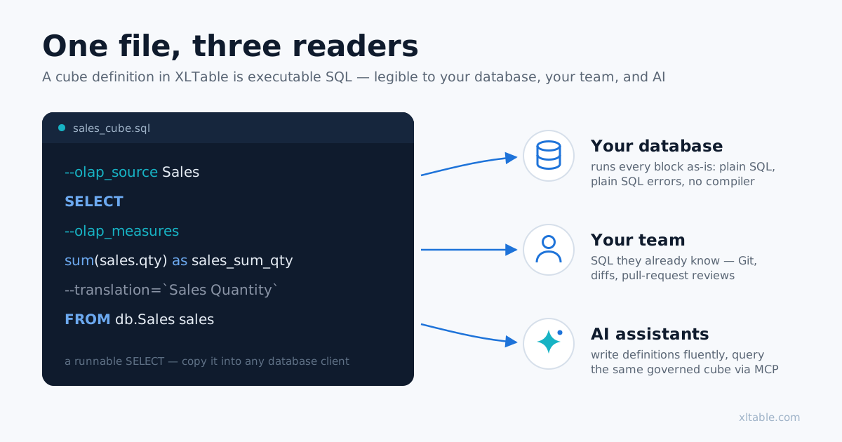
One file, three readers

Let's sum up. A semantic layer does not have to be a separate platform with its own modeling language, compiler, and learning curve. It can be a SQL file — one that can be read, executed, and version-controlled.

A cube definition in XLTable is equally legible to three very different readers. The database — because every block runs as is. The human — because it's SQL the data team already knows, with no new system of concepts. The AI — because a model can both write such definitions fluently and query data through them, losing neither the semantics nor the access controls.

And business users never see any of these layers at all. They open Excel, refresh the PivotTable, and get numbers that agree.

Don't take our word for any of this. Take a sample dataset, define the same metric both ways, and see which one you'd rather debug, review, and hand to an AI.

You can try it in about an hour: the Quickstart walks you from installing the server to your first PivotTable, and ready-made sample datasets are available for all eight supported databases — from ClickHouse to DuckDB. Documentation: xltable-olap.readthedocs.io. Questions: help@xltable.com.